
Sample Size for Paired t Test
Menu location: Analysis_Sample Size_Paired t.
This function gives you the minimum number of pairs of subjects needed to detect a true difference DELTA in population means with power POWER and two sided type I error probability ALPHA (Dupont, 1990; Pearson and Hartley, 1970).
Information required
- POWER: probability of detecting a true effect.
- ALPHA: probability of detecting a false effect (two sided: double this if you need one sided).
- DELTA: difference in population means.
- SD: estimated standard deviation of paired response differences.
Practical issues
- Usual values for POWER are 80%, 85% and 90%; try several in order to explore/scope.
- 5% is the usual choice for ALPHA.
- SD is usually estimated from previous studies.
- If possible, choose a range of mean differences that you want to have the statistical power to detect.
Technical validation
The estimated sample size n is calculated as the solution of:
$\displaystyle n=\frac{(t_{n-1, \space \alpha/2}+t_{n-1, \space \beta})^2}{d^2}$
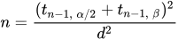
- where d = delta/sd, α = alpha, β = 1 - power and tv,p is a Student t quantile with v degrees of freedom and probability p. n is rounded up to the closest integer, then adjusted if necessary to the smallest n for which the power calculated from the non-central t distribution reaches POWER.
Example
Suppose you plan a study of peak expiratory flow rate (PEFR) before and after a walk on a cold day, like the one in the paired t test example but looking for a smaller effect. You want to detect a mean fall of 20 L/min with 80% power at a two sided alpha of 5%, and from that earlier study you expect the standard deviation of the paired differences to be about 35 L/min. The figures are invented for this illustration.
To run this in StatsDirect select Paired t from the Sample Size section of the Analysis menu. Enter 20 as the difference of population mean from zero, 35 as the standard deviation of the paired differences, 80% as the power and 5% as alpha. Then run it again with 90% as the power.
For this example:
Sample size for a paired or single sample Student t test
Alpha = 0.05
Power = 0.8
Difference of mean from zero = 20
Standard deviation = 35
Estimated minimum sample size = 27 pairs
Degrees of freedom = 26
and with 90% power:
Alpha = 0.05
Power = 0.9
Difference of mean from zero = 20
Standard deviation = 35
Estimated minimum sample size = 35 pairs
Degrees of freedom = 34
Twenty-seven pairs of measurements would give an 80% chance of detecting a true mean fall of 20 L/min, and 35 pairs a 90% chance. The size is the smallest number of pairs for which the power of the paired t test, calculated from the non-central t distribution, reaches the power asked for.
 R code
This R code reproduces the example above. It needs no packages and was checked with R 4.6.1. Paste it into R, or save it as a script and run it.
# Sample size for a paired t test: the StatsDirect help example (an invented plan for
# a study of peak expiratory flow rate before and after a cold walk, like the paired t
# test example: a fall of 20 L/min to detect, sd of paired differences 35 L/min) in R
delta <- 20                               # difference in population means to detect
sdiff <- 35                               # sd of the paired response differences
target <- 0.8                             # power, the probability of detecting delta
alpha <- 0.05                             # two sided type I error probability

# power.t.test solves for the number of pairs at which the power of the two sided
# paired t test, from the non-central t distribution, equals the target. strict = TRUE
# counts rejections in both tails as the report does; the default counts only the tail
# on the side of delta, which seldom changes the whole number of pairs.
r <- power.t.test(delta = delta, sd = sdiff, sig.level = alpha, power = target,
                  type = "paired", strict = TRUE)
print(r)

# A whole number of pairs: the smallest whose power reaches the target (checked below)
n <- ceiling(r$n)
cat("Alpha =", alpha, "\n")
cat("Power =", target, "\n")
cat("Difference of mean from zero =", delta, "\n")
cat("Standard deviation =", sdiff, "\n")
cat("Estimated minimum sample size =", n, "pairs\n")
cat("Degrees of freedom =", n - 1, "\n")

# The report also checks that n is the smallest number of pairs whose power reaches the
# target: the two sided power with n pairs, from the non-central t distribution with
# n - 1 degrees of freedom and non-centrality delta / (sd / sqrt(n)), and with n - 1
six <- function(x) formatC(x, digits = 6, format = "f", drop0trailing = TRUE)
pw <- function(n) {
  tcrit <- qt(1 - alpha / 2, n - 1)
  ncp <- delta / (sdiff / sqrt(n))
  pt(tcrit, n - 1, ncp, lower.tail = FALSE) + pt(-tcrit, n - 1, ncp)
}
cat("Power with", n, "pairs =", six(pw(n)), "and with", n - 1, "pairs =",
    six(pw(n - 1)), "\n")

# The same plan with 90% power
r90 <- power.t.test(delta = delta, sd = sdiff, sig.level = alpha, power = 0.9,
                    type = "paired", strict = TRUE)
n90 <- ceiling(r90$n)
cat("Power = 0.9\n")
cat("Estimated minimum sample size =", n90, "pairs\n")
cat("Degrees of freedom =", n90 - 1, "\n")